7. Read mapping
7.1. Preface
In this section we will use our skill on the command-line interface to map our reads from the evolved line to our ancestral reference genome.
Note
You will encounter some To-do sections at times. Write the solutions and answers into a text-file.
7.2. Overview
The part of the workflow we will work on in this section can be viewed in Fig. 7.1.
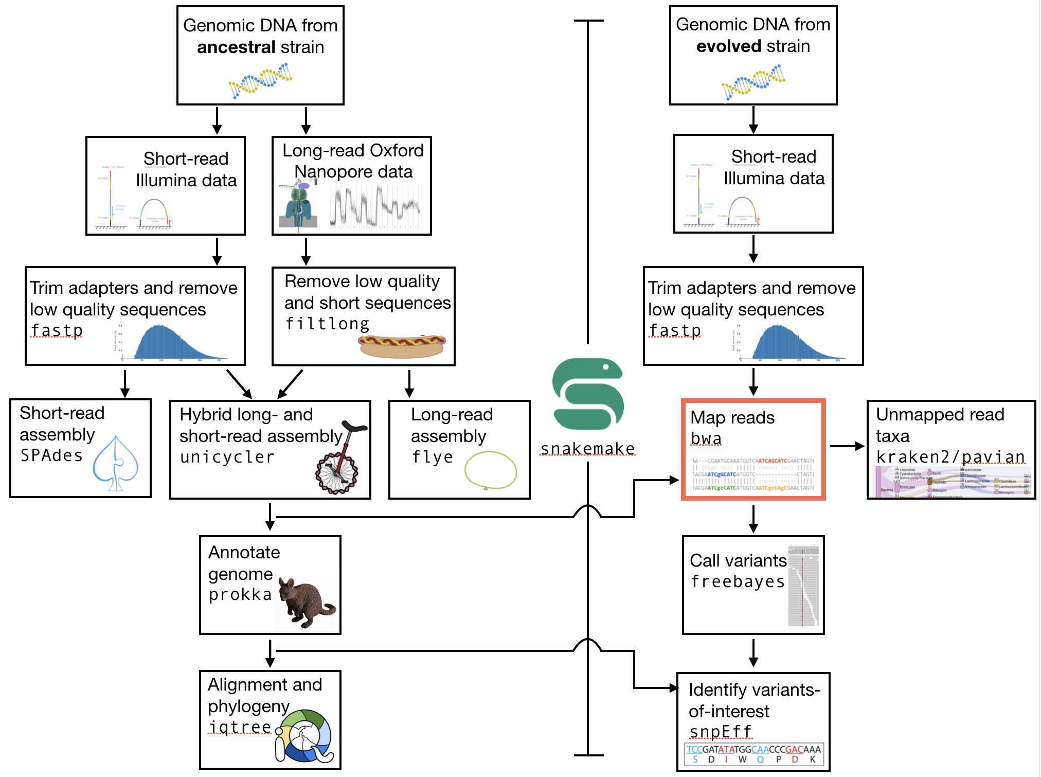
Fig. 7.1 The part of the workflow we will work on in this section marked in red.
7.3. Learning outcomes
After studying this section of the tutorial you should be able to:
Explain the process of sequence read mapping.
Use bioinformatics tools to map sequencing reads to a reference genome.
Filter mapped reads based on quality.
7.4. Before we start
Lets see what our directory structure looks like so far.
tree -L 2

# if we have used snakemake the structure
# should look similar to below
# with a data and results folder, and in the
# results folder there are trimmed reads and
# and assemblies
├── data
│   ├── illumina
│   └── nanopore
├── results
│   ├── H8_anc
│   ├── H8_anc_fastp.html
│   ├── H8_anc_fastp.json
│   ├── H8_anc.hiqual.fastq
│   ├── H8_anc_R1.trimmed.fastq
│   ├── H8_anc_R1.trimmed.sub.fastq
│   ├── H8_anc_R2.trimmed.fastq
│   └── H8_anc_R2.trimmed.sub.fastq
└── Snakefile
7.5. Mapping sequence reads to a reference genome
Now that we have assembled a reference genome for our ancestral clone, we want to identify the changes that have occurred in the evolved clone. There are at lteast two possible ways to do this. One option would be to assemble a second genome for our evolved clone and compare this to the ancestral genome. However, this would be the wrong approach for two reasons. First, it is more computationally difficult to peform another assembly. Thus, we would be wasting time and effort and computational resources. Second, we would not get any measure of how sure we could be that a change occurred. For these reasons we will instead map our reads onto the genome that we have assembled in the section Genome assembly. We will then figure out which mutations have occurred. This process is often denoted calling vraiants.
To map reads and call variants we will now use the second set of Illumina reads that you have, those from the evolved clone. Make sure that those are the ones you are dealing with today. First, we will go through the process of mapping them, and then we will add a rule to our snakefile that spceifies the input and output files tht we need, and the method used to create them.
First, you need to make sure that the reads you are using have been trimmed using fastp. If they are not, please go ahead and do that. For reference on how to use fastp, see QC section Quality control or refer to your snakefile.
We are going to use the quality trimmed forward and backward DNA sequences of the evolved line and use a program called BWA to map the reads.
7.6. BWA
7.6.1. Overview
BWA is a versatile read aligner that can take a reference genome and map single- or paired-end data to it [LI2009]. The method that it uses for this is the Burrows-Wheeler transform, and it was one of the first read aligners to adopt this strategy (with bowtie).
BWA first requires an indexing step for which you need to supply the reference genome. In subsequent steps this index will be used for aligning the reads to the reference genome. The general command structure of the BWA tools we are going to use are shown below:
# bwa index help
bwa index

# This is just indexing
# You only need your Unicycler assembly here
bwa index path/to/reference-genome.fasta

# bwa mem help
bwa mem

# paired-end mapping, general command structure, adjust to your case
# name you file SENSIBLY
# For this you need your ancestor assembly and your reads
# from your evolved lines
bwa mem path/to/reference-genome.fasta path/to/read1.fastq path/to/read2.fastq > path/to/aln-pe.sam
Create an BWA index for your reference genome assembly now using the bwa index command. Attention! Remember which file you need to submit to BWA.
Attention
If you have not used your Unicycler assembly as your reference, go back and do that now.
Attention
If you are writing the bwa index and bwa mem steps as rules in your Snakefile, this will be a little bit tricky. This is because the bwa index step has no explicit output. For this reason you need to generate an empty (fake) output. This can be done as illustrated below. Note that what we are doing is creating an empty file using touch(). All this does is tell us that the indexing has been done and that it has worked on the current assembly. And Remember to UPDATE your rule all :)
rule index:
  input:
    "results/my_assembly.fasta"
  output:
    touch("results/index.done")
  shell:
    """
    bwa index {input}
    """
Attention
(continued from above). Once you have done this, you will need to use this file (index.done) as input for your next mapping rule (probably something like bwa_mapping), like so:
rule bwa_mapping:
  input:
    assembly="results/my_assembly.fasta",
    R1="results/{strain}_R1.fastq",
    R2="results/{strain}_R2.fastq",
    index="results/index.done"
  output:
    "results/{strain}_mapped.sam"
  shell:
    """
    bwa mem {input.assembly} {input.R1} {input.R2} > {output}
    """
7.6.2. Mapping reads in a paired-end manner
Now that we have created our index, it is time to map the filtered and trimmed sequencing reads of our evolved line to the reference genome. Use the correct bwa mem command structure from above and map the reads of the evolved line to the reference genome. This process will take 2-3 minutes to complete.
7.7. The sam mapping file-format
BWA will produce a mapping file in sam format (Sequence Alignment/Map). Have a look into the sam-file that was created by either program.
A quick overview of the sam format can be found here.
Briefly, first there are a set of header lines for each file detailing what information is contained in the file. Then, for each read, that mapped to the reference, there is one line with information about the read in 12 different columns.
The columns of such a line in the mapping file are described in Table 7.1.
Col |
Field |
Description |
|---|---|---|
1 |
QNAME |
Query (pair) NAME |
2 |
FLAG |
bitwise FLAG |
3 |
RNAME |
Reference sequence NAME |
4 |
POS |
1-based leftmost POSition/coordinate of clipped sequence |
5 |
MAPQ |
MAPping Quality (Phred-scaled) |
6 |
CIAGR |
extended CIGAR string |
7 |
MRNM |
Mate Reference sequence NaMe (‘=’ if same as RNAME) |
8 |
MPOS |
1-based Mate POSition |
9 |
ISIZE |
Inferred insert SIZE |
10 |
SEQ |
query SEQuence on the same strand as the reference |
11 |
QUAL |
query QUALity (ASCII-33 gives the Phred base quality) |
12 |
OPT |
variable OPTional fields in the format TAG:VTYPE:VALUE |
One line of a mapped read can be seen here:
M02810:197:000000000-AV55U:1:1101:10000:11540 83 NODE_1_length_1419525_cov_15.3898 607378 60 151M = 607100 -429 TATGGTATCACTTATGGTATCACTTATGGCTATCACTAATGGCTATCACTTATGGTATCACTTATGACTATCAGACGTTATTACTATCAGACGATAACTATCAGACTTTATTACTATCACTTTCATATTACCCACTATCATCCCTTCTTTA FHGHHHHHGGGHHHHHHHHHHHHHHHHHHGHHHHHHHHHHHGHHHHHGHHHHHHHHGDHHHHHHHHGHHHHGHHHGHHHHHHFHHHHGHHHHIHHHHHHHHHHHHHHHHHHHGHHHHHGHGHHHHHHHHEGGGGGGGGGFBCFFFFCCCCC NM:i:0 MD:Z:151 AS:i:151 XS:i:0
Mpst importantly, this line defines the read name, the position in the reference genome where the read maps, and the quality of the mapping.
7.8. Mapping post-processing
7.8.1. Fix mates and compress
Because aligners can sometimes leave unusual SAM flag information on SAM records, it is helpful when working with many tools to first clean up read pairing information and flags with SAMtools.
We are going to produce also compressed bam output for efficient storing of and access to the mapped reads. To understand why we are going to compress the file, take a look at the size of your original fastq files that you used for mapping, and the size of the sam file that resulted. Along the way toward compressing, we will also sort our reads for easier access. This simply means we will order the reads by the position in the genoome that they map to.
To perform all of these steps, we will rely on a powerful quite of software tools that are implemented in samtools. The first of these, then is sort. One very important aspect of samtools that you should always remember is that in almost all cases the default behaviour of ``samtools`` is to output to the terminal (standard out). For that reason, we will be using the redirect arrow > quite a bit. In other cases, we will use the “pipe” operator |. We use the pipe operator so that we do not have to deal with intermediate files.
First, we use samtools fixmate, which according to its documentation, can be used to: “Fill in mate coordinates, ISIZE and mate related flags from a name-sorted or name-collated alignment.” Here, ISIZE refers to insert size.
Note, samtools fixmate expects name-sorted input files, which we can achieve with samtools sort -n.
# -n sorts by name
# -O sam outputs sam format
samtools sort -n -O sam my_mapped_file.sam > my_mapped_sorted.sam
Next, we need to take this name-sorted by and give it to samtools fixmate . This will fill in our extra fields. We will also output in compressed .bam format.
-m: Add ms (mate score) tags. These are used by markdup (below) to select the best reads to keep.-O bam: specifies that we want compressed bam output from fixmate.
# -O bam outputs bam format
samtools fixmate -m -O bam my_mapped_sorted.sam my_mapped_fixmate.bam
Attention
Make sure that you are following the file naming conventions for your suffixes. Simple mapped files will be in .sam format and should be denoted by that suffix. The compressed version will be in .bam format, and be denoted by that suffix.
Once we have this fixmate bam-file, delete the .sam files as they take up a significant amount of space. Use rm to do this, but be careful because ``rm`` is forever.
We will be using the SAM flag information later below to extract specific alignments.
Hint
A very useful tools to explain samtools flags can be found here.
7.8.2. Sorting by location
We are going to use SAMtools again to sort the .bam file into coordinate order:
# sort by location
# -O indicates bam output again
# note the redirect > arrow
samtools sort -O bam my_mapped_fixmate.bam > my_mapped_sorted.bam
7.8.3. Remove duplicates
In this step we remove duplicate reads. The main purpose of removing duplicates is to mitigate the effects of PCR amplification bias introduced during library construction. It should be noted that this step is not always recommended. It depends on the research question. In SNP calling it is a good idea to remove duplicates, as the statistics used in the tools that call SNPs sub-sequently expect this (most tools anyways). However, for other research questions that use mapping, you might not want to remove duplicates, e.g. RNA-seq.
# Markdup can simply *mark* the duplicate reads
# But the -r option tells it to remove those reads.
# the -S also tells it to remove supplementary mappings
# This works on a very simple principal that we will discuss
samtools markdup -r -S my_mapped_sorted.bam my_mapped_sorted_dedup.bam
7.8.4. Sequencing bias ToDo
Todo
Exlpain what “PCR amplification bias” means and discuss why removing duplicates to mitigate the effects of PCR amplification bias might not be used for RNA-seq experiments.
7.9. Mapping statistics
7.9.1. Stats with SAMtools
Lets get a mapping overview. For this we will use the samtools flagstat tool, which simply looks in your bam file for the flags <http://broadinstitute.github.io/picard/explain-flags.html> of each read and summarises them. The usage is as below:
samtools flagstat my_mapped_sorted_dedup.bam
7.9.2. Read mapping ToDo
Todo
Look at the mapping statistics and understand their meaning. Discuss your results.
For the sorted bam file we can also get read depth for at all positions of the reference genome, e.g. how many reads are overlapping the genomic position. We can get some very quick statistics on this using samtools coverage. Type that command to view the required input, and try using that now.
We can also get considerably more detailed data using samtools depth, used as below. Again note that here, as with almost all commands above, we are using the redirect > arrow.
samtools depth my_mapped_sorted_dedup.bam > my_mapping_depth.txt
This will give us a file with three columns: the name of the contig, the position in the contig, and the depth. This looks something like this:
# let's look at the first ten lines using head
head my_mapping_depth.txt

1 1 97
1 2 97
1 3 99
1 4 99
1 5 100
1 6 100
1 7 103
1 8 103
1 9 104
1 10  107
Now we quickly use some R to get some stats on this data. Skip this section if you are short on time.
Open an R shell by typing R on the command-line of the shell.
# here we read in the data
my.depth <- read.table('my_mapping_depth.txt', sep='\t', header=FALSE)

# Look at the beginning of x
# to make sure we've loaded it correctly
head(my.depth)

# calculate average depth
mean(my.depth[,3])
# std dev
sd(my.depth[,3])

# a quick pdf of coverage
# here we look at contig 1 and only plot eavery 100th point
# Please excuse this briefly complicated syntax
# every 100th point
plot.points <- seq(min(my.depth[,2]), max(my.depth[,2]),by=100)
pdf('my_depth.pdf', width = 12, height = 4)
plot(my.depth[plot.points,2], my.depth[plot.points,3], pch=19, xlab='Position', ylab='Coverage')
dev.off()
The result plot will be looking similar to the one in Fig. 7.2
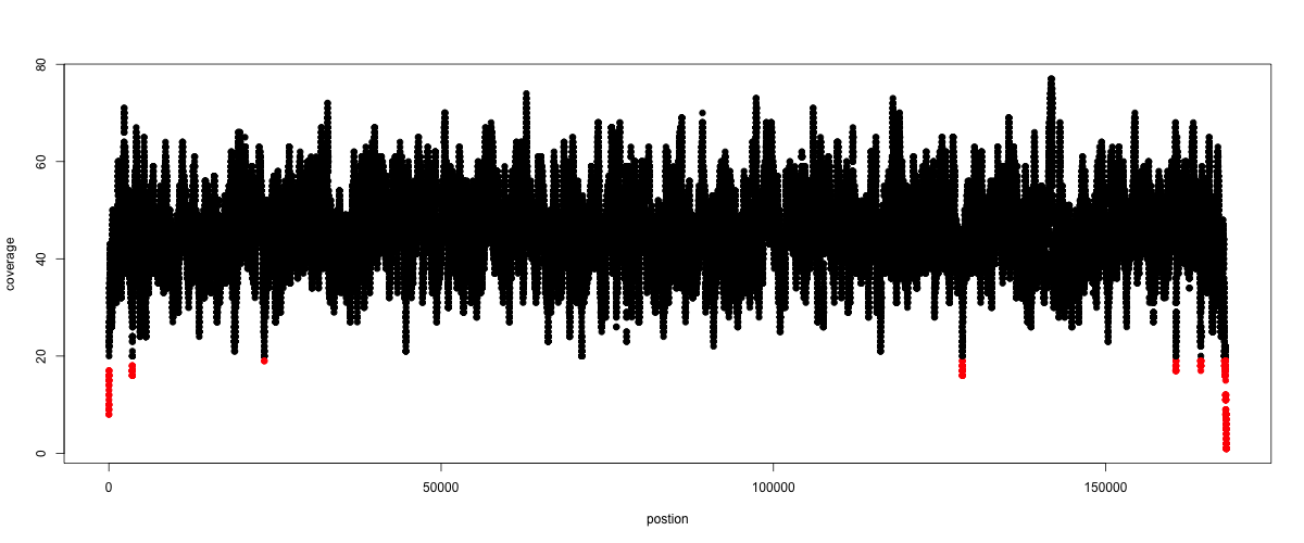
Fig. 7.2 A example coverage plot for a contig with highlighted in red regions with a coverage below 20 reads.
7.9.3. Stats with QualiMap
For a more in depth analysis of the mappings, one can use QualiMap [OKO2015].
QualiMap examines sequencing alignment data in SAM/BAM files according to the features of the mapped reads and provides an overall view of the data that helps to the detect biases in the sequencing and/or mapping of the data and eases decision-making for further analysis.
Installation:
conda install qualimap
Run QualiMap with:
qualimap bamqc -bam my_mapped_sorted_dedup.bam
This will create a report in the mapping folder. The name of this report will be similar to my_mapped_sorted_dedup_stats
See this webpage to get help on the sections in the report.
7.10. Sub-selecting reads
It is important to remember that the mapping commands we used above, without additional parameters to sub-select specific alignments (e.g. for Bowtie2 there are options like --no-mixed, which suppresses unpaired alignments for paired reads or --no-discordant, which suppresses discordant alignments for paired reads, etc.), are going to output all reads, including unmapped reads, multi-mapping reads, unpaired reads, discordant read pairs, etc. in one file.
We can sub-select from the output reads we want to analyse further using SAMtools.
7.10.1. Concordant reads
We can select read-pair that have been mapped in a correct manner (same chromosome/contig, correct orientation to each other, distance between reads is not non-sensical). For this, we will use another samtools utility, view, which converts between bam and sam format. We do this here because it outputs to standard out, and we extract reads that have the correct flag.
samtools view -h -b -f 3 my_mapped_sorted_dedup.bam > my_mapped_sorted_dedup_concordant.bam
-h: Include the sam header-b: Output will be bam-format-f 3: Only extract correctly paired reads.-fextracts alignments with the specified SAM flag set.
7.10.2. Read characteristics ToDo
Todo
Explain what concordant and discordant read pairs are? Look at the Bowtie2 manual.
7.10.3. Variant identification ToDo
Todo
Our final aim is to identify variants. For a particular class of variants, it is not the best idea to only focus on concordant reads. Why is that?
7.10.4. Quality-based sub-selection
Finally, in this section we want to sub-select reads based on the quality of the mapping. It seems a reasonable idea to only keep good mapping reads. As the SAM-format contains at column 5 the \(MAPQ\) value, which we established earlier is the “MAPping Quality” in Phred-scaled, this seems easily achieved. The formula to calculate the \(MAPQ\) value is: \(MAPQ=-10*log10(p)\), where \(p\) is the probability that the read is mapped wrongly. However, there is a problem! While the MAPQ information would be very helpful indeed, the way that various tools implement this value differs. A good overview can be found here. The bottom-line is that we need to be aware that different tools use this value in different ways and the it is good to know the information that is encoded in the value. Once you dig deeper into the mechanics of the \(MAPQ\) implementation it becomes clear that this is not an easy topic. If you want to know more about the \(MAPQ\) topic, please follow the link above.
For the sake of going forward, we will sub-select reads with at least medium quality as defined by Bowtie2. Again, here we use the samtools view tool, but this time use the -q option to select by quality.
samtools view -h -b -q 20 my_mapped_sorted_dedup_concordant.bam > my_mapped_sorted_dedup_concordant.q20.bam
-h: Include the sam header-q 20: Only extract reads with mapping quality >= 20
Hint
I will repeat here a recommendation given at the source link above, as it is a good one: If you unsure what \(MAPQ\) scoring scheme is being used in your own data then you can plot out the \(MAPQ\) distribution in a BAM file using programs like the mentioned QualiMap or similar programs. This will at least show you the range and frequency with which different \(MAPQ\) values appear and may help identify a suitable threshold you may want to use.
7.10.5. Unmapped reads
We will use Kraken2 in section Taxonomic investigation to classify all unmapped sequence reads and identify the species they are coming from and test for contamination. To achieve this we need to figure out which reads were unmapped, and then extract the sequence of those reads.
Lets see how to get the unmapped portion of the reads from the bam-file:
samtools view -b -f 4 my_mapped_sorted_dedup.bam > my_mapped_sorted_dedup_unmapped.bam

# count them
samtools view -c my_mapped_sorted_dedup_unmapped.bam
-b: indicates that the output is BAM.-f INT: only include reads with this SAM flag set. You can also use the commandsamtools flagsto get an overview of the flags.-c: count the reads
Lets extract the fastq sequence of the unmapped reads for read1 and read2. We will use this next time to figure out what organisms these reads might come from. Note that there are several complications here: we output to fastq format, and we separate into R1 and R2. Here we use a new tool, bamToFastq. This is part of the bedtools suite of tools, and of course for that we first need to install bedtools using conda :) . Go ahead and do that now.
Finally, we extract the fastq files:
bamToFastq -i my_mapped_sorted_dedup_unmapped.bam -fq my_mapped_sorted_dedup_unmapped.R1.fastq -fq2 my_mapped_sorted_dedup_unmapped.R2.fastq
References
- TRAPNELL2009
Trapnell C, Salzberg SL. How to map billions of short reads onto genomes. Nat Biotechnol. (2009) 27(5):455-7. doi: 10.1038/nbt0509-455.
- LI2009
Li H, Durbin R. (2009). Fast and accurate short read alignment with Burrows-Wheeler transform. Bioinformatics. 25 (14): 1754–1760.
- OKO2015
Okonechnikov K, Conesa A, García-Alcalde F. Qualimap 2: advanced multi-sample quality control for high-throughput sequencing data. Bioinformatics (2015), 32, 2:292–294.