5. Genome assembly
5.1. Preface
In this section we will use our skill on the command-line interface to create a genome assembly from sequencing data. We will constructing three types of assebmlies: A short-read only assembly (with Illumina data); a long-read only assembly (with Oxford Nanopore data); and a “hybrid” assembly (using both Illumina and Oxford Nanopore data).
Note
You will encounter some To-do sections at times. Write the solutions and answers into a file (MS Word, Google docs, or any text editor).
5.2. Overview
The part of the workflow we will work on in this section can be viewed in Fig. 5.1.
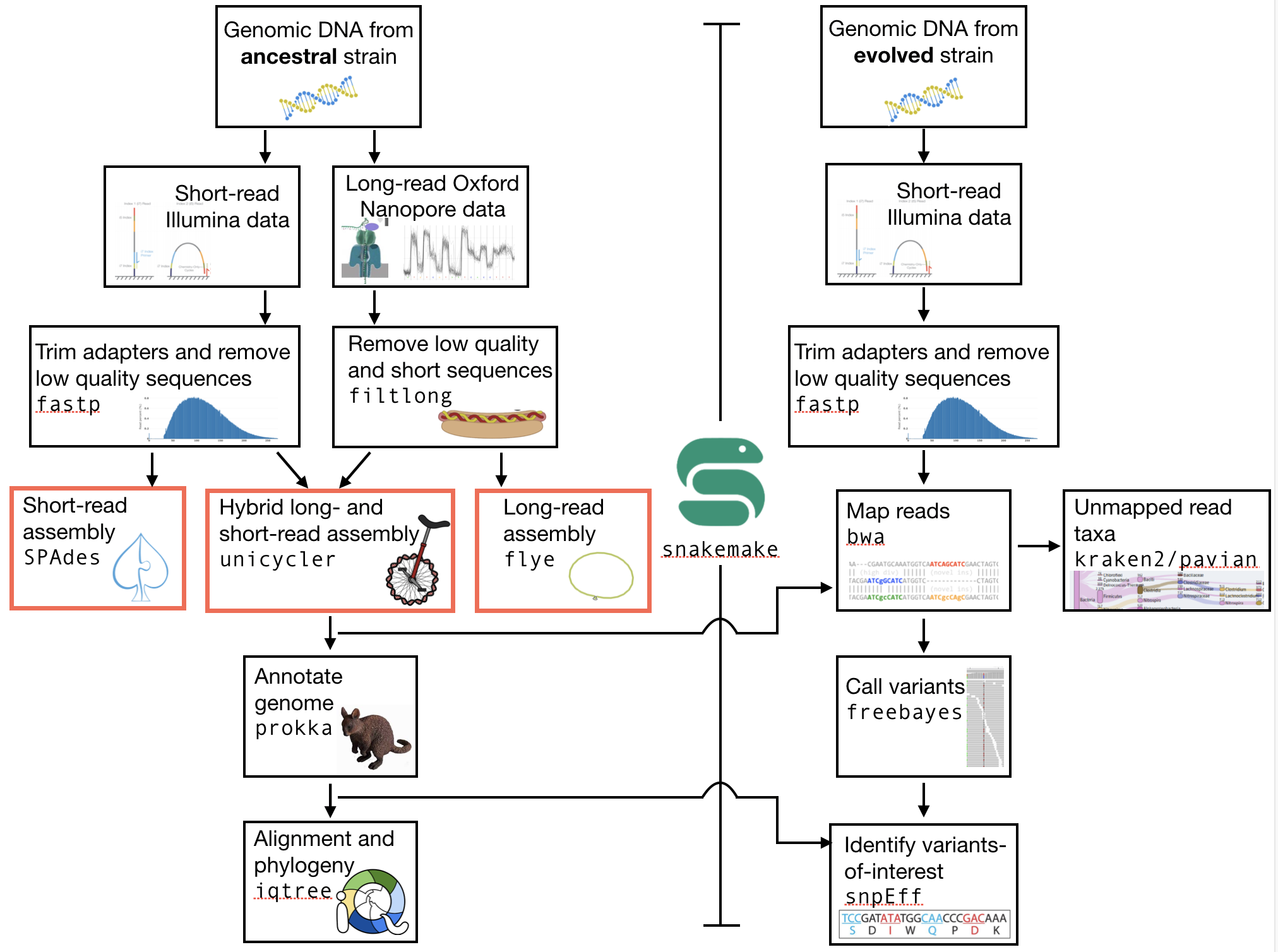
Fig. 5.1 The part of the workflow we will work on in this section marked in red.
5.3. Learning outcomes
After studying this tutorial you should be able to:
Construct and interpret a whole genome assembly.
Discuss the relative advantages and disadvantages of using short- and long-read seqeuncing technology for genome assembly.
Judge the quality of a genome assembly.
5.4. Before we start
Are your directories organised and clean?
tree -L 2
And let’s make sure we have our conda environment activated:
conda activate ngs
5.4.1. Subsampling reads
Due to the size of the short read Illumina data set, you may find that it takes a lot of time for the assembly to complete, especially on older hardware.
To mitigate this problem we will randomly select a subset of sequences to use at this stage of the tutorial.
To do this we will install the program seqtk. Use conda install to install this program now.
Now that you have installed seqtk, you are going to sample the original Illumina reads so that you have at most 50X coverage. To do this, we will again estimate the bacterial genome size as 5 Mbp, meaning that 50X coverage would require a total of 250 Mbp of data. If you have less than this, you do not need to subsample. However, most of you will have more than this. For this reason, we will select only some of these to use for assembly. You can check how many Mbp of data you have right now by using the program that you installed previously, seqkit. Remember that the command in seqkit that gives you a summary of your .fastq file data is seqkit stats. Go ahead and remind yourself of the content of your trimmed .fastq files for your ancestor dataset. Next, some calculations.
First note that there are three arguments that we are giving to seqtk, all of which can be seenif you type seqtk sample at the command line. The arguments are:
#. a “seed”, which determines what random subset of reads are selected (i.e. it is fed into a random number generator)
#. a file of reads (trimmed)
#. the fraction or number of reads to maintain.
For this latter argument, the easiest to use is probably the fraction. You will need to calculate this number. For example, if the seqkit stats summary says that you have a total of 750 Mbp of data, and you would like 250 Mbp, then you will need to sample 1/3 of the reads. In general the fraction you need to sample would be: 250Mpb / total_bp. Calculate this fraction now.
The seed (-s11 in the command below) determines how the random number generator begins. It is critical that the seed you set for subsampling is the same for both sets of reads. However, you are free to change the seed itself (e.g. you could use -s100 for both readsets if you want). Using a different seed from your neighbour may have the interesting downstream effect of giving you slightly different genome assemblies. Anyway, onto the sampling itself. The command you will use will be similar to:
# Subsample reads.
# Note the redirect arrow. Without this, the reads will
# simply be output to your terminal screen
seqtk sample -s11 my.reads_R1.trimmed.fastq 0.2 > my.sub.reads_R1.trimmed.fastq.gz
seqtk sample -s11 my.reads_R2.trimmed.fastq 0.2 > my.sub.reads_R2.trimmed.fastq.gz
Note
To repeat: the -s options needs to be the same value for file 1 and file 2 to sample the reads that match with each other. -s specifies the seed value for the random number generator. If you have not done this, repeat the command.
Note
It is true that by reducing the amount of reads that go into the assembly, we are losing information that could otherwise be used to make the assembly. Thus, the assembly may become worse (although this is by no means certain).
5.5. Keeping processes going - tmux usage
The assembly programs that we will use today will take some time to complete because they are solving very difficult problems. However, you will want to make sure that the programs keep running even after you have logged out of the server and quit your VM. The tmux program allows exactly this - you can keep processes (i.e. software programs) operating in the background so that they continue running after you have logged out from a server. This can be extremely useful for programs that take a while to complete. To use tmux, simply type tmux at the command prompt. This will bring you to a new screen. If you find that tmux is not installed, go ahead and install it with conda.
The single most important thing to remember about tmux is that to do anything to control the window, you must type <ctrl>-b first. If you do not do this, you will simply keep typing on the command line. There are only four basic commands to remember:
<ctrl>-b(move into control mode)<ctrl>-b d(Detach from the current session and return to the normal command line)<ctrl>-b x(eXit from the current session and quit it to return to the normal command line)When on the normal command line:
tmux ls. This will list all the currenttmuxsessions you have, by name.When on the normal command line:
tmux a -t session_name. This will return (Attach) you to thetmuxsession that you specify withsession_name
Once you are in your new tmux screen, you can go ahead and start running your software.
5.6. Creating a genome assembly
We want to create a genome assembly for our ancestor strain. We are first going to make a short-read only assembly using the subsampled and quality trimmed R1 and R2 Illumina sequences. We will use a program called SPAdes to build a genome assembly.
5.6.1. Reference genome ToDo
Todo
Discuss briefly why we are using the ancestral sequences to create a reference genome as opposed to the evolved line.
5.6.2. Installing the short-read assembly software
The intallation of SPAdes can be done through conda, although the program should be specificed as spades. Go ahead and install the program now.
5.6.3. SPAdes usage
# to get a help for spades and an overview of the parameters type:
spades.py -h
The two files we need to submit to SPAdes are two paired-end read files. We also need to specify the output location with -o. Before you continue with the assembly command, make sure you are using tmux.
The command you use will be something similar to:
spades.py -o output_dir -1 input.R1.fastq -2 input.R2.fastq
Next go ahead and detach from the tmux session using <ctrl>-b d. This should bring you back to the normal command line. You can check that your tmux session is running by typing tmux ls. You can also check your activity on the server by typing: htop -u myusername. This should bring up the htop window and show that you are running a SPAdes assembly. To quit htop, type q.
5.6.4. Installing the long-read assembly software
We are next going to make a long-read only assembly using the quality filtered Oxford Nanopore reads. We will use a program called Flye to build a long-read genome assembly. This can be installed using conda. The name of the program is simply flye. Go ahead and install it now.
5.6.5. Flye usage
For flye we only need a single file of reads - the long Oxford Nanopore reads. We will also need to specify the type of reads (a long-read assembler could use another type of long read, such as PacBio), the estimated genome size, and the number of threads to use. Please do not use more than two threads!
Again, you will do this in a tmux terminal, as the assembly will take some time to complete. Open up a new tmux terminal now by typing tmux at the command line. Once you have that open, go ahead and start the assembly using a command similar to:
flye --nano-raw my_longreads.fastq --out-dir myassembly_long \
--genome-size 5m --threads 2
Here, 5m refers to the genome size in Megabase pairs.
5.6.6. Assembly ToDo
Todo
List one advantage and one disdvantage each for long-read and short-read assemblies.
5.6.7. Installing the hybrid assembly software
Finally, we are going to perform a hybrid assembly. For this, we will use both the short-read Illumina data and the long-read Oxford Nanopore data. By combining the data, we will be able to exploit the strengths of each - the accuracy of the Illumina data and the length of the Oxford Nanopore data. This should give you a more accurate assembly than using either readset alone. The program you will use to perform the hybrid assembly is Unicycler. This program can be installed using conda. Go ahead and do that now. It should be specified as unicycler.
5.6.8. Unicycler usage
Unicycler can be run using a command that is similar to the programs above, although we will need to specify both the long- and short-read datasets. Below I am writing the command over two lines (and thus using \) so that you do not need to scroll. You can do the same; if so, press <enter> following the \. You can also simply type the hoel command on one line.
unicycler -1 my_short_reads_R1.fastq -2 my_short_reads_R2.fastq.gz -l my_long_reads.fastq -o my_output_dir
Go ahead and run Unicycler now.
Attention
As with the other assembly programs, Unicycler can take a while to run. For this reason, you should run it using tmux. If yoou have noot started it in a tmux terminal, please stop the assembly now by typing <ctrl>-c, open up a new tmux terminal, and restart the assembly. Remember that to exit the tmux terminal, you will have to type <ctrl>-b d.
5.7. Assembly quality assessment
To gain an intuitive and qualitative unbderstanding of assembly quality, we will simply visualise the assemblies. We will be able to compare the quality more precisely in a later lab in which we annotate the genome with the locations of the open reading frames, tRNAs, rRNAs, and other genomic elements. We will discuss in lecture why more standard assembly metrics, such as N50 or L50, are not useful for bacterial assemblies anymore (as opposed to the situation only two or three years ago).
5.7.1. Assembly visualisation
We are going to use a piece of software called Bandage to visualise the assemblies. This was also written by Ryan Wick, the author of Filtlong and Unicycler. While Bandage can be used as a graphical user interface program, here we are going to use it via the command line, and then simply download the results. You can use conda to install it. It is located on the bioconda channel and is called, simply, bandage. Install it now.
Bandage visualises the graph of an assembly - the contigs and the connections or overlaps between the contigs; see here for an explanation. These overlaps are areas of the assembly that cannot be resolved because there are multiple identical or nearly identical sequences (kmers) in the genome, and the assembler cannot decide which sequence is attached to which other sequence. Assembly graphs are most commonly saved in a format called .gfa (for details see here).
To use Bandage you will direct it to the .gfa files from your assembly.
To see the usage for bandage, you can type Bandage --help (note that there is an uppercase B in bandage). The option you should use is something similar to:
# Below, specify your .gfa file and the name of the
# image you want to output to, usually ending in .png or .jpg
Bandage image myfile.gfa myfile.png
You can then use scp or rsync to copy this image file down to your own desktop. I recommend rsync using syntax similar to the following:
# Be very careful and precise about which directory you are copying from
# and your login name and the IP address. Note that here I have used
# the * wildcard character to match any file that ends in ".gfa"
rsync -az --progress mylogin@remote.server.IP:~/mydir/assemblydir/*.png ./
Do this for all of your assemblies - the short-read only, long-read only, and hybrid assemblies. Once you have copied all of those to your VM desktop, go ahead and open Bandage and load the graphs. Again, for details on how to do this, see the instructions here.
5.7.2. Assembly comparison ToDo
Todo
Compare the visualisations of your long-read only and hybrid assemblies. Do they look similar? Describe the results of the visualisation in detail (e.g. the number of contigs, the size of the contigs, etc.)
Contrast the results of your long-read and hybrid assemblies with your short-read only assembly. What is the major difference between the short-read only assembly and the other two?
5.8. Further reading
5.8.1. Background on Genome Assemblies
How to apply de Bruijn graphs to genome assembly. [COMPEAU2011]
Sequence assembly demystified. [NAGARAJAN2013]
5.8.2. Evaluation of Genome Assembly Software
GAGE: A critical evaluation of genome assemblies and assembly algorithms. [SALZBERG2012]
Assessment of de novo assemblers for draft genomes: a case study with fungal genomes. [ABBAS2014]
5.9. Web links
Bandage (Bioinformatics Application for Navigating De novo Assembly Graphs Easily) is a program that visualizes a genome assembly as a graph [WICK2015].
References
- ABBAS2014
Abbas MM, Malluhi QM, Balakrishnan P. Assessment of de novo assemblers for draft genomes: a case study with fungal genomes. BMC Genomics. 2014;15 Suppl 9:S10. doi: 10.1186/1471-2164-15-S9-S10. Epub 2014 Dec 8.
- COMPEAU2011
Compeau PE, Pevzner PA, Tesler G. How to apply de Bruijn graphs to genome assembly. Nat Biotechnol. 2011 Nov 8;29(11):987-91
- NAGARAJAN2013
Nagarajan N, Pop M. Sequence assembly demystified. Nat Rev Genet. 2013 Mar;14(3):157-67
- WICK2015
Wick RR, Schultz MB, Zobel J and Holt KE. Bandage: interactive visualization of de novo genome assemblies. Bioinformatics 2015, 10.1093/bioinformatics/btv383